Generalised Additive Models - mgcv (WIP)
A replication of the ecological models per Hierarchical generalized additive models in ecology: an introduction with mgcv using stock data.
Packages and data
Load the required packages and the standard data set for analysis
library(romerb)
library(mgcv)
library(gratia)

data("stock_data")
fundamental_raw <- stock_data
rm(stock_data)

# Data
df <- fundamental_raw[fundamental_raw$date_stamp == as.Date('2021-06-30'), ]
df$log_mkt_cap <- log(df$mkt_cap)
df$log_book <- log(-df$total_equity_cln)
df$roe <- df$roe * -1
df <- df[df$date_stamp == as.Date('2021-06-30'), c('symbol','sector','log_book','log_mkt_cap','log_pb','roe','leverage')]
Hierachical GAM (model type GS)
Using the factor smooth basis.
# Model
gam_mlm1 <- gam(
  log_pb ~ s(roe, k = 5, m = 2) + s(roe, sector, k = 5, m = 2, bs = "fs"),
  data = df,
  method = "REML"
  )

# Predict
gam_mlm1_pred <- predict(gam_mlm1, se.fit = TRUE)
df$pred <- gam_mlm1_pred$fit
df$sepred <- gam_mlm1_pred$se.fit

# Visualise
ggplot(data = df, aes(x = roe, y = log_pb, group = sector)) +
  facet_wrap(~reorder(sector, as.numeric(sector)), ncol = 4, scales = 'free') +
  geom_ribbon(aes(ymin = pred - 2 * sepred,
                  ymax = pred + 2 * sepred), alpha=0.25) +
  geom_line(aes(y = pred)) +
  geom_point(alpha = 0.3) +
  labs(x = 'Return on equity',
       y = 'Log price / book ratio')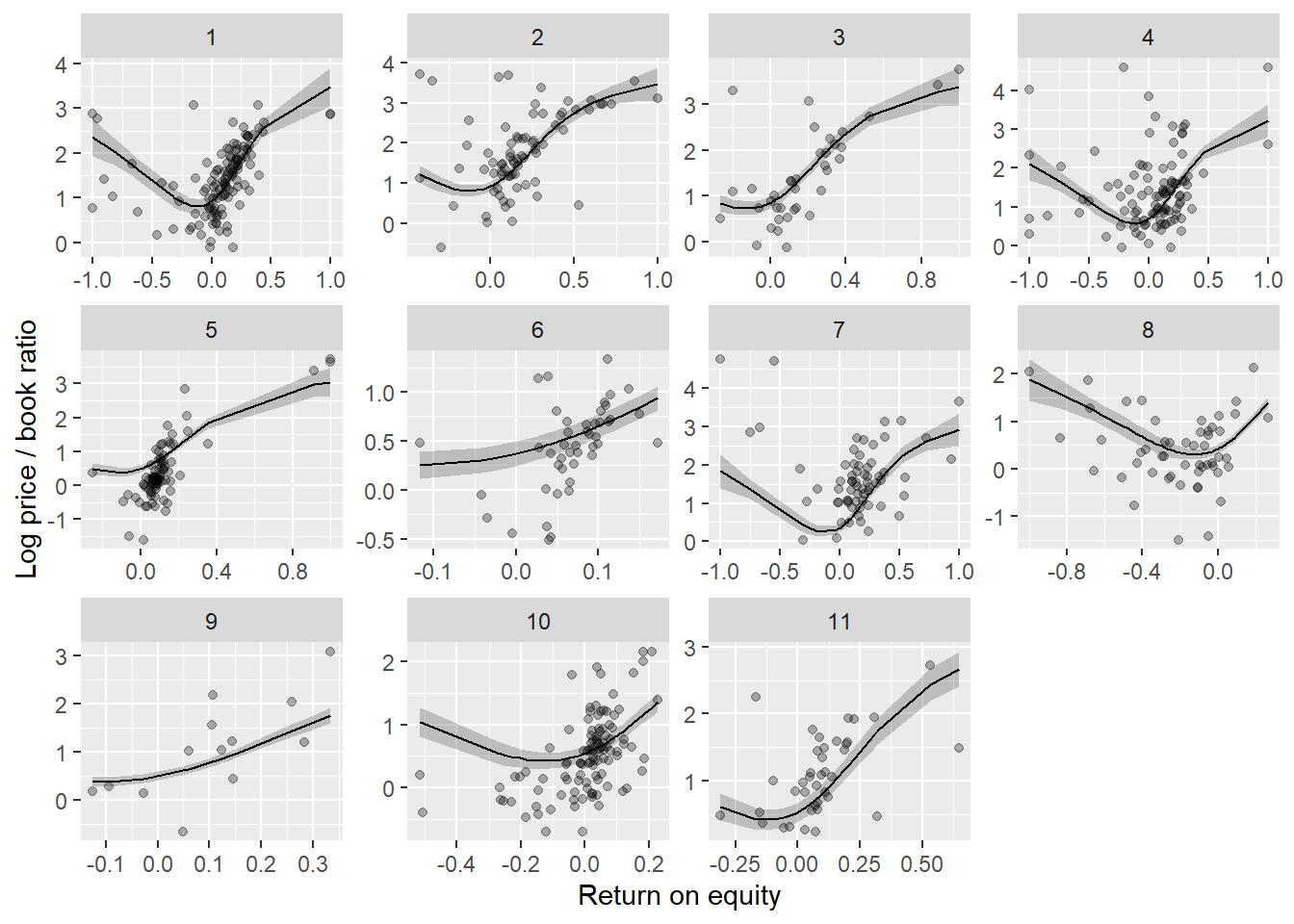
Non-hierachical & 3d visualisation
# Model
gam_mlm2 <- gam(
  log_pb ~ s(roe, leverage, bs = "tp", k = 5, m = 2), #+ s(roe, sector, k = 5, m = 2, bs = "fs"),
  data = df,
  method = "REML"
  )

# Predict
interval <- 30
roe <- with(df, seq(min(roe), max(roe), length = interval))
leverage <- with(df, seq(min(leverage), max(leverage), length = interval))

new_data <- expand.grid(roe = roe, leverage = leverage)

gam_mlm2_pred <- matrix(predict(gam_mlm2, new_data), interval, interval) #, type = "response"


# Visualise
# https://bikeactuary.com/datasci/gams_scams_pt1
persp(
  x = leverage,
  y = roe,
  zlab = 'log_pb',
  gam_mlm2_pred, theta = 225, phi = 20, col = "blue", ticktype = "detailed")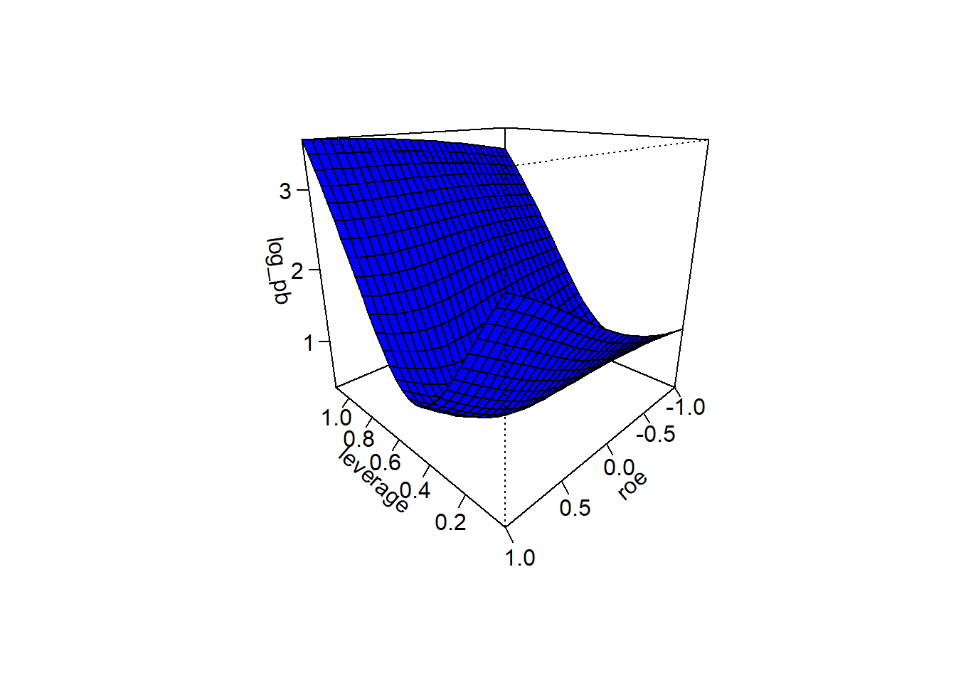
Single level interaction model
Using a tensor product smooth. Modelling market capitalisation on return on equity and book value of equity.
# Model
gam_te1 <- gam(
  log_mkt_cap ~ te(roe, log_book, bs=c("cc", "tp"), k=c(10, 10)),
  data = df, method = "REML"
  )

# Visualise
gratia::draw(gam_te1)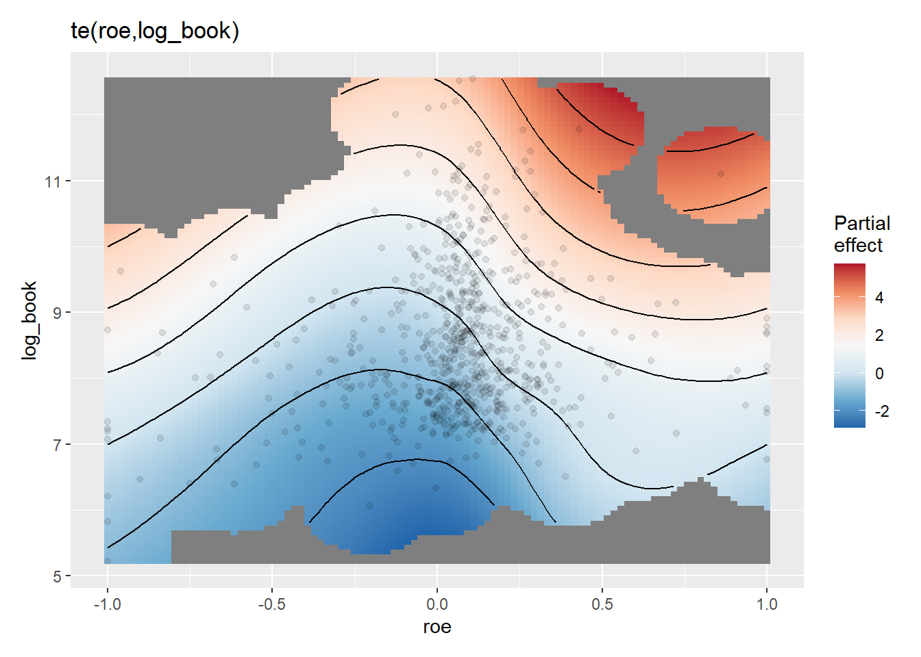
Same model, visualise with a 3d plot.
# Predict
interval <- 30
roe <- with(df, seq(min(roe), max(roe), length = interval))
log_book <- with(df, seq(min(log_book), max(log_book), length = interval))

new_data <- expand.grid(roe = roe, log_book = log_book)

gam_te1_pred <- matrix(predict(gam_te1, new_data), interval, interval)

# Visualise
persp(
  x = log_book,
  y = roe,
  zlab = 'log_mkt_cap',
  gam_te1_pred, theta = 45, phi = 20, col = "blue", ticktype = "detailed")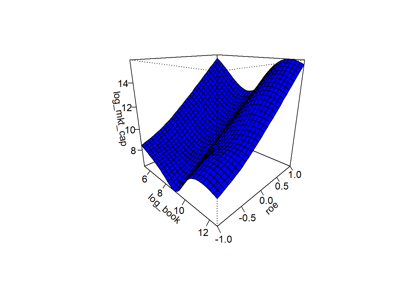
Modelling price to book ratio on return on equity and leverage.
gam_te2 <- gam(
  log_pb ~ te(roe, leverage, bs=c("cc", "tp"), k=c(10, 10)),
  data = df, method = "REML"
)

gratia::draw(gam_te2)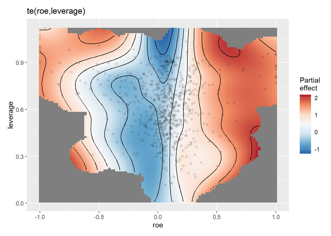
Same model, visualise with a 3d plot.
# Predict
interval <- 30
roe <- with(df, seq(min(roe), max(roe), length = interval))
leverage <- with(df, seq(min(leverage), max(leverage), length = interval))

new_data <- expand.grid(roe = roe, leverage = leverage)

gam_te2_pred <- matrix(predict(gam_te2, new_data), interval, interval)

# Visualise
persp(
  x = leverage,
  y = roe,
  zlab = 'log_pb',
  gam_te2_pred, theta = 225, phi = 20, col = "blue", ticktype = "detailed")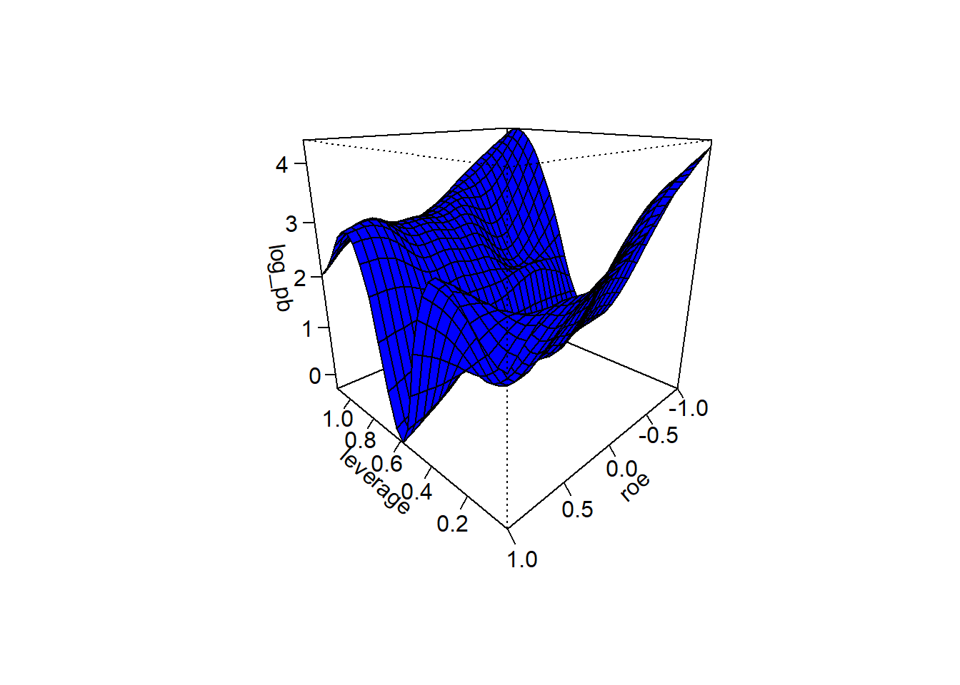
Once again using plotly.
References
3d plots with color
https://stackoverflow.com/questions/22652941/how-to-add-colorbar-with-perspective-plot-in-r https://stackoverflow.com/questions/31374951/add-points-and-colored-surface-to-locfit-perspective-plot https://stackoverflow.com/questions/24918604/how-to-have-only-every-other-border-in-a-persp https://stackoverflow.com/questions/3786189/r-4d-plot-x-y-z-colours