Gaussian Process regression - base R
A replication of the Gaussian Process regression implementation from chapter 5 of Surrogates. Application of the same code to real data.
Chapter example
Data
Create some dummy data being an independent and dependent variable, along with a grid of the independent variable values.
# Training data
n <- 8
X <- matrix(seq(0, 2*pi, length=n), ncol=1)         # independent variable
y <- sin(X)                                         # dependent variable

# Predictive grid
XX <- matrix(seq(-0.5, 2*pi + 0.5, length=100), ncol=1)
Covariance function / kernel
Using inverse exponentiated squared distance.
Note that the first three lines below can be replicated with
D <- plgp::distance(X).
D <- dist(X, diag = T, upper = T)
D <- D**2
D <- as.matrix(D)                            # euclidean distance
eps <- sqrt(.Machine$double.eps)             # nugget / jitter
Sigma <- exp(-D) + diag(eps, ncol(D))        # exponentiated squared euclidean distance
Multi-variate normal conditioning
Covariance of testing grid data points.
DXX <- as.matrix(dist(XX, diag = T, upper = T)**2)  # Is this the same as plgp::dist?
SXX <- exp(-DXX) + diag(eps, ncol(DXX))
Covariance between testing grid and training data.
Kriging equations, mean mup and variance
Sigmap.
Posterior/predictive distribution
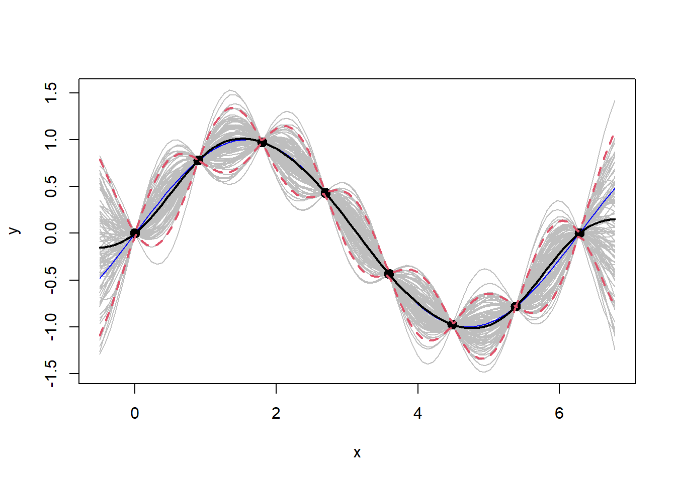
Generate Y values from the posterior/predictive distribution and plot.
YY <- rmvnorm(100, mup, Sigmap)
# Error bars
q1 <- mup + qnorm(0.05, 0, sqrt(diag(Sigmap)))
q2 <- mup + qnorm(0.95, 0, sqrt(diag(Sigmap)))
# Plot
matplot(XX, t(YY), type="l", col="gray", lty=1, xlab="x", ylab="y")
points(X, y, pch=20, cex=2)
lines(XX, sin(XX), col="blue")
lines(XX, mup, lwd=2)
lines(XX, q1, lwd=2, lty=2, col=2)
lines(XX, q2, lwd=2, lty=2, col=2)
Stock data example
The procedures above are now applied to real data, that being stock valuations and fundamentals.
Data
library(romerb)
data("stock_data")
fundamental_raw <- stock_data
rm(stock_data)
# Medical devices sector only
df <- fundamental_raw[fundamental_raw$sector == 7, ]
df$log_mkt_cap <- log(df$mkt_cap)
df$log_book <- log(-df$total_equity_cln)
df <- df[df$date_stamp == as.Date('2021-06-30'), c('log_book','log_mkt_cap','log_pb','roe','leverage')]
# nugget / jitter
eps <- sqrt(.Machine$double.eps)
# Training data
X <- matrix(df$roe)
y <- matrix(df$log_pb)
# Predictive grid
XX <- matrix(seq(min(X), max(X), length=200), ncol=1)
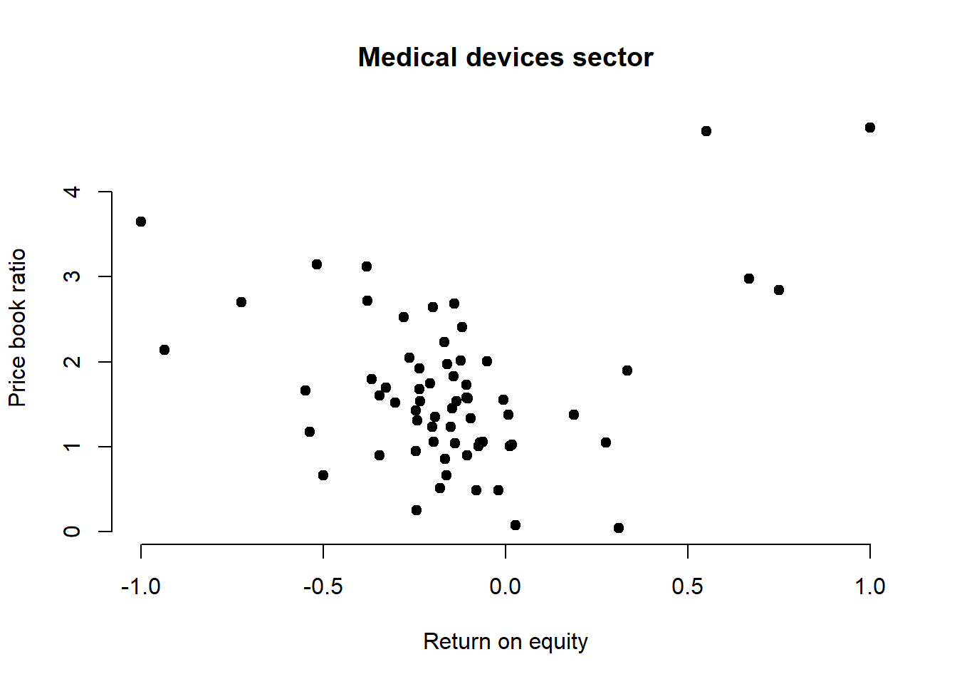
# Plot
plot(X, y, main = "Medical devices sector",
xlab = "Return on equity", ylab = "Price book ratio",
pch = 19, frame = FALSE)
Covariance function / MVN conditioning
D <- plgp::distance(X)
Sigma <- exp(-D) + diag(eps, length(X))
DXX <- plgp::distance(XX)
SXX <- exp(-DXX) + diag(eps, length(XX))
SX <- exp(-distance(XX, sort(X))) # note the sort, required to construct symmetric matrix at Sigmap
# Kriging equations, mean mup and variance Sigmap
Si <- solve(Sigma)
mup <- SX %*% Si %*% y
Sigmap <- SXX - SX %*% Si %*% t(SX)
Sigmap <- sfsmisc::posdefify(Sigmap, method = "allEVadd")
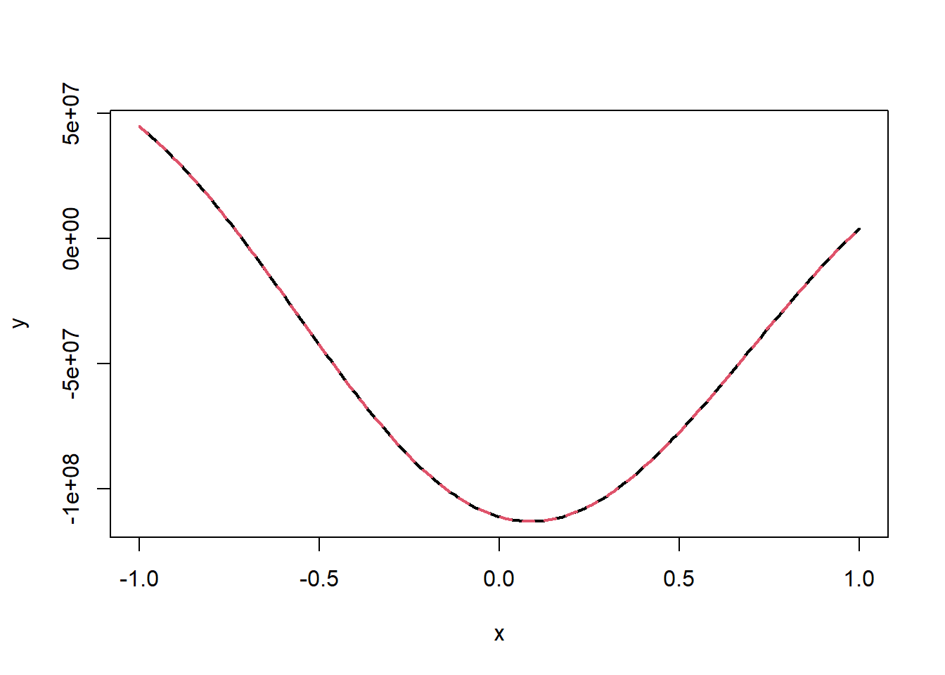
# Generate Y values & error bars from the posterior/predictive distribution
YY <- rmvnorm(100, mup, Sigmap)
q1 <- mup + qnorm(0.05, 0, sqrt(diag(Sigmap)))
q2 <- mup + qnorm(0.95, 0, sqrt(diag(Sigmap)))